The Sampling Agents' Equilibrium

It's Sunday morning, the weather is good, and you want to get some work done over a cup of coffee at 36 Cake Cafe. One thing stands between you and the decision: how busy will the cafe be?

To decide, you gather some data. You remember last Sunday you had glanced at the bar from across the street. Maybe you text a friend who lives near the cafe. Based on that evidence you determine whether you'd end up with a nice seat by the window and a peaceful morning and decide to go, or that it'd be bustling so you stay home.

The cafe's actual demand is being decided simultaneously by hundreds of others across town.

While this serves as a fun toy example of a coordination problem, it is a powerful metaphor for the impending scale of autonomous agents and their impact on the macro economy.

Between the rising adoption of agents like OpenClaw and Hermes Agent, the rollout of agentic commerce infrastructure by financial giants like Stripe¹1Stripe. Stripe Agentic Commerce, Mastercard²2Mastercard. Mastercard Agent Pay, and American Express³3American Express. Agentic Commerce, and foundational market mapping by Microsoft Research⁴4Microsoft. Agentic Markets: Equilibrium Effects of Improving Consumer Search, we are firmly entering the era of true delegation. Agents will soon be transacting, negotiating, shopping, and optimizing our lives in the background.

This reality raises an important and fascinating question.

When millions of autonomous agents begin making decisions on our behalf:

How does the information they consume dictate aggregate behavior and shape the broader economy?

This isn't the first time agents and algorithms have quietly been used to run a massive market. Having spent most of my career engineering and optimizing ads bidding systems, I can foresee many structural parallels. Yet, many new inventions and challenges will undoubtedly surface. The biggest differentiator in this world is that now everyone's agents will be participating in this broader decision and data market.

This is taking the already complex ads marketplace to the $N$th degree.

This blog introduces the core ideas of sampling equilibrium with statistical inference (SESI) by Salant and Cherry⁵5Salant, Y. and Cherry, J. Statistical Inference in Games, Econometrica (2020) to understand how a decentralized system settles into different steady states from the information they are able to obtain.

Elements of a decision#

Everyone interested in going to the cafe has a private upside. Perhaps it's how much you like their lattes, how close it is, or how well you work there. And at the same time, no one likes a packed cafe.

We put this into notation in the table below.

Symbol	Note
$\alpha \in [0,1]$	Participation — the fraction of the population that goes. The one aggregate quantity everybody is trying to guess.
$\theta \sim H$	Idiosyncratic benefit — how much you want to go. Distributed uniformly on $[0,1]$ across the population.6
$f(\alpha)$	Crowding cost — increasing and convex, the same for everyone. Domain and range $\in [0,1]$.7
$\theta > f(\alpha)$	Decision rule — go if your private benefit clears the crowding cost.
$k$	Sample size — how many observations someone gets; their data budget / how well-informed they are.
$J \sim \mathrm{Bin}(k,\alpha)$	Positive count — how many of those $k$ observations were "going." The estimate is $\hat\alpha = J/k$.

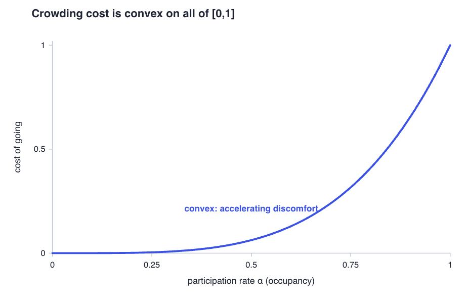
For our example, we will consider $f(\alpha) = \alpha^4$.

The problem with crowds#

Suppose you had a magic ball that told you the true participation rate $\alpha$. Then the population behavior is obvious: everyone with $\theta > f(\alpha)$ goes, everyone else stays home. With our uniform distribution over $\theta$,

$$\text{fraction staying home} = f(\alpha)$$

So the fraction who go is $1-f(\alpha)$, aka the response map,

$$1 - f(\alpha)$$

The problem is, there is no magic ball. Precisely because $\alpha$ isn't a fact about the world, it is the aggregation of decisions by each person using what they know about how busy the cafe will get.

It becomes a chicken and egg problem. Everyone thinks to themselves that they'll go if it's not too crowded, but if everyone thinks that way then everyone will go. If everyone goes, then no one will want to go. Ad infinitum.

Equilibrium#

A silver lining: self-consistency and self-regulation#

The way out requires us to stop thinking about a true $\alpha$ and start looking for an $\alpha$ that is self-consistent and self-enforcing — a level of busyness which, if everyone believed it, would produce exactly that level of busyness.

That is, the fraction staying home is $1-\alpha$, and the fraction staying home is also $f(\alpha)$. So we need

$$1 - \alpha = f(\alpha)$$

In this case, we have a Nash equilibrium since everyone would have perfect information about the crowdedness.

Existence and Uniqueness: The left side falls from 1 to 0 as $\alpha$ goes from 0 to 1; the right side climbs from $f(0)$ to $f(1)$. Two continuous curves going opposite directions cross once.

To make this concrete, suppose that everyone gathers at the cafe at the break of dawn, joining the queue in order from greatest benefit to least. Naturally, as the line forms, people who are intolerant of crowdedness will refrain from joining it. By the time the cafe opens, we would have our equilibrium — everyone who wanted to join would have joined, and no one in the queue would want to leave, since their derived utility already clears their decision rule. This is made possible because we mandated that people consider joining the queue in decreasing utility order.

SESI & Iterated Equilibrium#

Reality is, not everyone is willing to walk by the cafe without an idea of its crowdedness. People usually go based on an estimate.

Estimation & Imperfect Information#

We can model a person's estimate of the participation rate as $k$ independent observations of other people (e.g. did this one go, or not), from which they compute the obvious estimate:

$$\hat\alpha = J/k, \qquad J \sim \mathrm{Bin}(k, \alpha)$$

$k$ describes how well-informed someone is. $k=1$ is "I asked one guy." $k=30$ is "I have a decent read." $J$ denotes the number of successes in the sample of $k$ observations. As $k$ grows the estimate tightens around the truth.

Crucially, people then act on $\hat\alpha$ as that is their best estimate. They go if $\theta > f(\hat\alpha)$⁸8We use the maximum likelihood estimator throughout this post, though the framework works for any inference procedure. Details are in Salant and Cherry⁵.. Different people draw different samples, which introduces variance to the population.

For instance, if there were $j$ goers in a sample of $k$, the expression below is the fraction of people who observe $j$ successes and decide that they should stay home:

$$f(\tfrac{j}{k}) \quad \times \underbrace{\binom{k}{j}\alpha^{j}(1-\alpha)^{k-j}}_{\text{Pr($J$ successes in $k$ trials with prob $\alpha$)}}$$

To find out what the population does, we need to sum over that variation:

$$\operatorname{Bern}_k(\alpha; f) := \mathbb{E}_J\big[f(\hat\alpha)\big] = \sum_{j=0}^{k} f\!\left(\tfrac{j}{k}\right)\binom{k}{j}\alpha^{j}(1-\alpha)^{k-j}$$

This is the Bernstein operator, and despite the notation it is nothing but an expectation. It takes the cost curve $f$ and blurs it by exactly the amount of noise a $k$-sample estimate carries. Small $k$, heavy blur. Large $k$, almost no blur.

Two properties that matter:

1. Monotonicity. If $f$ increases in $\alpha$, so does $\operatorname{Bern}_k(\alpha;f)$.
2. Convexity. If $f$ is convex, then $\operatorname{Bern}_k(\alpha;f)$ is itself convex, and $\operatorname{Bern}_k(\alpha;f) \ge \operatorname{Bern}_{k+1}(\alpha;f) \ge f(\alpha)$, with strict inequality on the interior $0<\alpha<1$ when $f$ is not linear.

Property 2 plays a pivotal role in understanding SESI, so here's a dedicated widget to demonstrate it.

SESI#

Definition. A sampling equilibrium with statistical inference (SESI) is the participation fraction $\alpha_k$ that arises when individuals each draw $k$ observations from a Bernoulli distribution with probability of success $\alpha_k$ and best-respond to their estimate.

The self-reference is the core of the concept.⁹9It is worth noting that although in this blog post we describe the steady state interpretation of SESI via population evolution dynamics, SESI itself exists as a fixed point equilibrium. Instead of sampling from a magic urn as in theory land, agents sample one another according to their past history.

The equilibrium condition is the same as before with $f$ replaced by the Bernstein operator:

$$1 - \alpha = \operatorname{Bern}_k(\alpha; f),$$

and it has exactly one solution, for the same reason as before: a decreasing line meeting an increasing curve.

How uncertainty suppresses demand#

In the above sections, we defined SESI and the Bernstein operator with respect to a sampling budget $k$. The more samples you have, the more certain your estimate will be. In the limit as $k \to \infty$, SESI naturally approaches the Nash equilibrium, as you have perfect information.

And this increase is monotonic, as per Property 2 of the Bernstein operator!

Under our convex crowding cost function $f$, the more certainty we have about the estimate, the more demand the cafe will get!¹⁰10The opposite relation holds for concave cost functions.

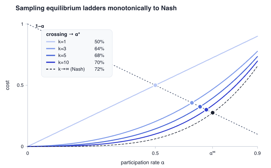
Every person's estimate of $\alpha$ is unbiased, and the town's average estimate is exactly correct. The bias shows up only after you push that estimate through the cost curve. With increasing marginal cost, being wrong by 20 points in the crowded direction inflates your expected cost more than being wrong by 20 points in the empty direction deflates it.

This is just Jensen's inequality applied to our convex $f$. The expectation of the function sits above the function of the expectation:

$$\mathbb{E}\big[f(\hat\alpha)\big] \;>\; f\big(\mathbb{E}[\hat\alpha]\big) \;=\; f(\alpha)$$

The last equality shows the unbiasedness: guessing crowdedness is fair, but pricing it is not. Everyone is right on average about how busy the cafe is, and everyone still expects it to be worse than it is. Uninformed crowds under-participate.

The $k=1$ example is a nice sanity check: someone who asks one person concludes either "nobody's going" or "everybody's going," and the town lands on exactly a coin flip. That holds for any cost curve with $f(0)=0$ and $f(1)=1$ — with one observation, the shape of $f$ stops mattering entirely.

Equilibrium from iteration dynamics#

We've discussed the estimation process and how uncertainty hurts participation, but how does a population actually get to that equilibrium point?

Suppose the whole town re-samples every week using the previous week's information. Last Sunday it rained and the cafe was nearly empty — 20% went. So this week almost everyone goes: 99.8%. Which means next week almost nobody does.

$$0.20 \to 0.998 \to 0.006 \to 1.000 \to 0.000 \to \cdots$$

It oscillates, just like the chicken and egg problem.

Revolving Patrons and Amnesia#

Consider instead at the very beginning it was just a random guess for each person in town, and the agents observed some participation rate. Everyone heard how crowded it was.

But each week, not everyone is going to remember the crowdedness. Or maybe some fraction of the town breaks their routine, or moves out of the neighborhood. And in their stead, new people have come to town and found good reviews about the cafe.

Newcomers need to get an estimate of the crowdedness, perhaps from their neighbors or recent reviews on platforms. Some fraction of the townsfolk will fuzzily recall the crowdedness. They get an estimate, form a belief, and decide.

We put this into notation. But first recall the response map.¹¹11Given a believed participation rate, how much of the population actually shows up? With a magic oracle that was simply $1-f(\alpha)$ — everyone who clears the crowding cost goes. With sampling, each townsperson (with fuzzy memory) / newcomer draws $k$ observations, forms an estimate $\hat\alpha$, and goes iff $\theta>f(\hat\alpha)$. Averaging over that noise, the fraction that goes is

$$R(\alpha) \;=\; 1-\operatorname{Bern}_k(\alpha;f).$$

Call $R$ the sampling response map. Under perfect information ($k\to\infty$) one recovers $R(\alpha)=1-f(\alpha)$.

To reach a stable equilibrium, the system needs inertia.¹²12This is effectively a damping factor. In this example, only a fraction $\epsilon$ of the population re-evaluates their choice each period.

The paper gives a sufficient condition for reaching a steady state:

$$\epsilon < \frac{1}{1 + f'(1)}$$

where $\epsilon$ is the fraction of the population that samples each period.

We can read it as amnesia / turnover has to be slow relative to how sharply crowding hurts the experience. For $f(\alpha)=\alpha^4$ that threshold is exactly 1/5. The steeper the crowding penalty, the more inertia the system requires to arrive at a steady state. Inertia here is $1-\epsilon$, the proportion of people who don't resample.

We define our population's participation dynamics as the following: Each period a fraction $1-\epsilon$ of the population keeps last period's action, and a fraction $\epsilon$ re-samples and best-responds via $R$. The next generation's participation is therefore

$$\alpha_t = (1-\epsilon)\,\alpha_{t-1} + \epsilon\, R(\alpha_{t-1}) \;\equiv\; h(\alpha_{t-1}).$$

A steady state of $h$ is a fixed point $\alpha=R(\alpha)$, which is exactly the SESI condition $1-\alpha=\operatorname{Bern}_k(\alpha;f)$. The bound on $\epsilon$ is what makes $h$ a contraction toward that point rather than an oscillator around it.

Ultimately, equilibrium is a claim about the stable long run, and Salant and Cherry formulate the above process and demonstrate that it converges naturally to a SESI.

SESI Convergence Demo#

The widget below runs the $\epsilon$-replacement dynamic for $f(\alpha)=\alpha^4$. Drag $\epsilon$, $k$, and the starting $\alpha_0$ and watch whether the cafe equilibrium settles or cycles.

A few notes:

• The phase plot is drawn in response space — $R(\alpha)$ against $\alpha$, so the cobweb diagram is easier to follow.
• Blue and orange answer different questions. Blue is $R(\alpha_t)$: what the $\epsilon$-fraction who actually sample this period do. Orange is $h(\alpha_t)=\alpha_{t+1}$: what the whole town does, once you average those samplers against the $1-\epsilon$ who kept last week's habit. The town only ever moves an $\epsilon$-fraction of the way from $\alpha_t$ toward the blue curve, so the cobweb steps ride orange — blue is the target it is chasing, never a state the population occupies.
• The paper's bound $\epsilon<1/(1+f'(1))=0.20$ (the red mark) is only sufficient, and quite conservative. The real edge is where $h$ stops contracting, $\epsilon<2/(1+\operatorname{Bern}_k'(\alpha_k))$ — the grey mark. It sits near $0.8$ for most sample sizes, but runs all the way to $1$ at $k=1$, where the response map is a straight line and the dynamic settles for every $\epsilon$.
• Lastly, starting belief $\alpha_0$ is any initial belief participation rate that we start our cafe at. Therefore, in the diagram, it always lands on the blue curve to start. Following that, the population dynamics takes over, which is why it follow the orange line afterwards.

Concluding Remarks#

SESI formalized how the amount of information each agent receives is a lever on controlling the market's outcome, a lever separate from anyone's preferences or the underlying economics. Nobody has to be fooled or persuaded; where the equilibrium is settled is determined by uncertainty (or lack of it) alone.

In a variation of their model, Salant and Cherry note how a monopolist is mathematically incentivized to intentionally withhold information. By artificially widening the information gap, they obscure who actually owns a luxury good. This protects its perceived exclusivity and, in turn, elevates demand.

Viewed from another angle, SESI informs us about how we can steer the economy by information design alone.

This holds profound implications for the agentic era. We assume we are entering a time of abundant information, yet we increasingly see platforms gatekeeping their data behind closed doors. How this flow of information is controlled will determine how economies move.

And just as search engines and ad networks optimized what human eyeballs saw to drive conversions, undoubtedly the information giants will play a role in optimizing what agents see.

And SESI is just one piece of the puzzle. As we delegate our economic agency to agents and algorithms, mechanism and information design will become the defining challenges of the agentic era.

---

What's Next:

My ongoing research and interest is at the intersection of AI, algorithmic game theory, and mechanism design. More to come soon.

If you're researching or building in this space or adjacent areas and want to collaborate or trade notes, drop a line in my inbox and let's connect.

@article{feng2026sesiprimer,
  title   = {The Sampling Agents' Equilibrium},
  author  = {Feng, Terry},
  journal = {terryfeng.io},
  year    = {2026},
  month   = {Aug},
  url     = {https://terryfeng.io/writing/sesi-primer}
}